Quantum Hall Effect
Quantum Hall Effect
A quantum state in two dimensions
2D electron gas in strong perpendicular magnetic fields.
Can exist for bosons too!
Landau Levels
- Single particle Hamiltonian with vector potential
H = -\frac{1}{2m}\left(\nabla -i q \mathbf{A}\right)^2
- For perpendicular field
\partial_x A_y - \partial_y A_x = B
- We choose symmetric gauge
A_x = -\frac{1}{2} B y,\quad A_y = \frac{1}{2} B x
H in complex coordinates
\begin{aligned} z &= x + i y, \quad \bar z = x - iy\\ \partial_z &= \frac{1}{2}\left(\partial_x - i\partial_y\right), \quad \partial_{\bar z} = \frac{1}{2}\left(\partial_x + i\partial_y\right)\\ H &= -\frac{2}{m}\left(\partial_z -\frac{qB \bar z}{4}\right)\left(\partial_{\bar z} +\frac{qB z}{4}\right) + \frac{\omega_c}{2} \end{aligned}
- \omega_c = \frac{qB}{m} is the cyclotron frequency
Lowest Landau level
H = A^\dagger A + \frac{\omega_c}{2}
- The operator A is defined as
A \equiv i \sqrt{\frac{2}{m}}\left(\partial_{\bar z} +\frac{qBz}{4}\right)
- Notice that z^\dagger = \bar z while (\partial_{\bar z})^\dagger = -\partial_z
States that satisfy \left(\partial_{\bar z} +\frac{qB z}{4}\right)\psi(z,\bar z) = 0 have energy \omega_c/2
Since \langle{\psi}\rvert A^\dagger A \lvert \psi \rangle\geq 0 these belong to the lowest Landau level (LLL)
Check
Show that these states have the form
\psi(z,\bar z) = f(z) \exp\left(-\frac{qB}{4}\left|z\right|^2\right)
where f(z) is an arbitrary analytic function.
f(z)=a_0 + a_1z + a_2 z^2+\ldots for arbitrary a_n
Landau levels highly degenerate
Notation
- Write LLL wavefunction as f(z), leaving Gaussian in inner product
\langle{f_1}\rvert f_2\rangle = \int \frac{d^2z}{2\pi} \overline{f_1(z)}f_2(z) \exp\left(-\left|z\right|^2/2\right)
Units with magnetic length \ell \equiv (qB)^{-1/2}=1
A possible orthonormal basis is f_n(z) = \frac{z^n}{\sqrt{2^n n!}}
Check
Show this
Filled LLL of Fermions
Lift degeneracy by adding harmonic potential V_\text{harm}(x,y) = \frac{v}{2}\left(x^2+y^2\right) = \frac{v}{2}\left|z\right|^2
Problem: V_\text{harm}(z,\bar z)f(z) is not in LLL
Consider only the action of V in the LLL subspace
Check
By considering matrix elements \langle{f_1}\rvert V\lvert{f_2}\rangle between LLL states, show (by integrating by parts) that it is possible to replace any occurrence of \bar z in V with 2\partial_z acting on the analytic part of the wavefunction.
Note that the order is important: all the \partial_z must stand to the left of the z, Thus V_\text{harm}\longrightarrow v\partial_z z = v\left(1+z \partial_z\right)
- Applied to f_n(z), V just counts the degree: V_\text{harm} f_n = v(1+n)f_n
Fill states n=0,1,\ldots N-1
As for 1D fermions, single particle states are powers z^n.
Identical arguments imply
\Psi(z_1,\ldots, z_N) = \prod_{j<k}^N (z_j-z_k) \exp\left(-\frac{1}{4}\sum_{j=1}^N\left|z_j\right|^2\right)
Check
Show that the density is \rho_1(z,\bar z) = \frac{e^{-|z|^2/2}}{2\pi}\sum_{n=0}^{N-1} \frac{\left|z\right|^{2n}}{2^n n!} = \frac{1}{2\pi} \frac{\Gamma(N,|z|^2/2)}{(N-1)!} \Gamma(s,x) = \int^\infty_x t^{s-1}e^{-t}dt is incomplete gamma fn.
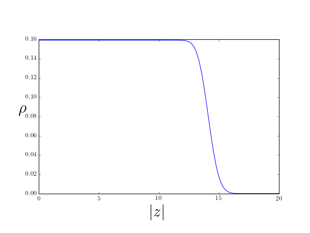
At small \left\|z\right\|, approximate by infinite sum, and \rho_1\to \frac{1}{2\pi}
The density is fixed at this value until we reach \sim\sqrt{2N}, then falls to zero on scale of \ell_B.
The filled LLL is described by a circular droplet of fixed density \rho_1 = 1/(2\pi): one state per flux quantum \Phi_0=2\pi/q
Changing confining potential causes the droplet to deform, but density to remain constant
The Laughlin Wavefunction
In 1983 Robert Laughlin proposed the generalization \Psi_m(z_1,\ldots, z_N) = \prod_{j<k}^N (z_j-z_k)^{m} \exp\left(-\frac{1}{4}\sum_{j=1}^N\left|z_j\right|^2\right)
m odd / even for fermions / bosons. m\neq 1 not a product state!
This Letter presents variational ground-state and excited-state wave functions which describe the condensation of a two-dimensional electron gas into a new state of matter.
m=2 boson state
With the repulsive potential H_{\text{int}} = g\sum_{j<k}\delta(\mathbf{r}_j-\mathbf{r}_k),\qquad g>0 m=2 state has zero interaction energy
Any state with zero interaction energy must have \Psi_2(z_1,\ldots, z_N) as a factor
If wavefunction has higher degree, then in the presence of potential V_\text{harm} it will have higher energy, so \Psi_2 is ground state
Particle distribution
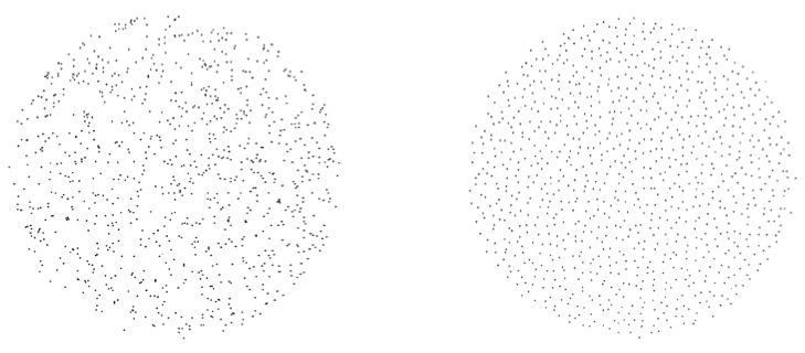
Monte Carlo samples from uncorrelated (uniform) distrubution vs. the Laughlin probability distribution \lvert\Psi_3(z_1,\ldots z_N)\rvert^2
Note uniformity of particle distribution, in contrast with the sample of uncorrelated particles on the left
The Plasma Analogy
- Probability distribution \lvert\Psi_m(z_1,\ldots, z_N)\rvert^2 of particles interpreted as Boltzmann distribution of particles in a classical 2D plasma
\nabla^2 V = -q\delta(\mathbf{r})
In 2D the solution describing a point charge is V_\text{point}(\mathbf{r}) = -\frac{q}{2\pi}\log\left|\mathbf{r}\right|
Constant background charge density -\rho_0 gives rise to a potential V_\text{bg}(\mathbf{r}) = \frac{\rho_0}{4} \left|\mathbf{r}\right|^2
System of identical charges in a background charge has overall electrostatic energy V(\mathbf{r}_1,\ldots,\mathbf{r}_N) = -\frac{q^2}{2\pi} \sum_{j<k}\log\left|\mathbf{r}_j-\mathbf{r}_k\right| + \frac{q\rho_0}{4}\sum_j \left|\mathbf{r}_j\right|^2
At finite temperature (unnormalized) probability of finding particles at locations \mathbf{r}_1, \ldots, \mathbf{r}_N is \exp[-\beta V(\mathbf{r}_1, \ldots, \mathbf{r}_N)] = \left|\Psi_m(\mathbf{r}_1, \ldots, \mathbf{r}_N)\right|^2 where we set \beta q^2/(2\pi) = 2m and \beta q\rho_0 = 2.
These are not physical electrostatic fields!
N\to\infty limit
- Introduce a continuum charge density \rho(\mathbf{r}) and write the energy as a functional \begin{aligned} \beta V[\rho] = -m\int d^2\mathbf{r}\, d^2\mathbf{r}'\rho(\mathbf{r})\log\left|\mathbf{r}-\mathbf{r}'\right|\rho(\mathbf{r}') + \frac{1}{2}\int d^2\mathbf{r}\left|\mathbf{r}\right|^2\rho(\mathbf{r}) \end{aligned}
Check
Show that minimizing the energy with respect to \rho(\mathbf{r}) – corresponding to finding the most likely configuration – leads to the condition -2m\int d^2\mathbf{r}'\log\left|\mathbf{r}-\mathbf{r}'\right|\rho(\mathbf{r}') + \frac{1}{2}\left|\mathbf{r}\right|^2 = 0
Check
Show that applying \nabla^2 to both sides gives \rho(\mathbf{r}) = \frac{1}{2\pi m}
Conclusion: density is fixed at 1/m of value for m=1 case
Result applies where density is non-zero, so we get a uniform droplet of radius \sqrt{2Nm}
1/m is called the filling fraction of the state.
Excited states: fractional charge
Simplest excited state is quasihole \begin{aligned} \Psi_\text{hole}(z_1,\ldots, z_N|Z) &= \left(\prod_j (Z-z_j)\right)\Psi_m(z_1,\ldots, z_N)\\ V(\mathbf{r}_1, \ldots, \mathbf{r}_N)&=-\frac{q^2}{2\pi m}\sum_j \log\left|\mathbf{r}_j-\mathbf{R}\right|-\frac{q^2}{2\pi} \sum_{j<k}\log\left|\mathbf{r}_j-\mathbf{r}_k\right|\\ &+ \frac{\rho q_0}{4}\sum_j \left|\mathbf{r}_j\right|^2 \end{aligned} `
Charge q/m at point \mathbf{R} = (X, Y), where Z=X+iY
Plasma will screen this charge, leaving a ‘hole’ in density distribution of charge -q/m
Hole state
- 20 holes with charge -20/m for clarity
Fractional Statistics
- Two quasihole wavefunction
\Psi_\text{2 hole}(z_1,\ldots, z_N|Z_1,Z_2) = \left(\prod_j (Z_1-z_j)(Z_2-z_j)\right)\Psi_m(z_1,\ldots, z_N)
\vert\Psi_\text{2 hole}(z_1,\ldots, z_N\vert Z_1,Z_2)\rvert^2 is plasma with two 1/m charges at positions \mathbf{R}_{1,2}
Each surrounded by depleted density of -1/m of a particle
(See notes) Quasiholes are anyons, particles with fractional statistics!